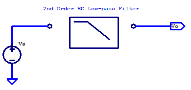
One of the simplest designs for a second order low-pass filter, is a RC ladder with 2 resistors and 2 capacitors. A drawback to this filters simplicity is that it requires a near ideal voltage source and a load with extremely high input impedance (ex. a buffer amplifier). A schematic of a second order RC low-pass filter is shown in the schematic below.

An intermediate filter potential \( V_x\) is added for analysis purposes only. To solve for the transfer function of \(V_s/V_o\), we begin with KCL at the \(V_x\) node as,
\[ \dfrac{V_x-V_s}{R_A} + V_xsC_A + \dfrac{V_x – V_o}{R_B} = 0 \tag{1} \]
KCL on the output node yields
\[ V_o s C_B + \dfrac{V_o – V_x}{R_B} = 0 \tag{2} \]
\[ V_o \left( sC_B + \dfrac{1}{R_B} \right) = \dfrac{V_x}{R_B} \tag{3}\]
\[ V_x \left(\dfrac{1}{R_A} + s C_A + \dfrac{1}{R_B} \right) = \dfrac{V_s}{R_B} + \dfrac{V_o}{R_B} \tag{4}\]
\begin{align*}
V_x &= \left( \dfrac{V_s}{R_A} + \dfrac{V_o}{R_B} \right) \dfrac{1}{1/R_A + sC_A + 1/R_B} \\
V_x &= \left( \dfrac{V_s}{R_A} + \dfrac{V_o}{R_B} \right) \dfrac{R_AR_B}{R_A + R_B + s R_A R_B C_A } \\
V_x &= \dfrac{ V_sR_B + V_o R_A}{R_A + R_B + s R_A R_B C_A } \tag{5}\\
\end{align*}
Substitution of (5) into (3) yields,
\[ V_o \left( sC_B + 1/R_B \right) = \dfrac{ V_sR_B + V_o R_A}{\left( R_A + R_B + s R_A R_B C_A \right) R_B } \tag{6}\]
\[R_B V_o \left( sC_B + 1/R_B\right) – \dfrac{V_oR_A}{R_A + R_B + s R_A R_B C_A} = \dfrac{V_sR_B}{R_A + R_B + sR_A R_B C_A} \tag{7}\]
\[ V_o \left( \dfrac{\left(sR_BC_B + 1 \right) \left( R_A + R_B + sR_AR_B C_A \right) }{R_A + R_B + s R_A R_B C_A} \right) = \dfrac{V_s R_B}{R_A + R_B + s R_A R_B C_A} \tag{8}\]
With some arrangement,
\[ \dfrac{V_o}{V_s} = \dfrac{R_B}{\left( sR_BC_B + 1\right)\left( R_A + R_B + s R_A R_B C_A \right) – R_A} \tag{9}\]
Collecting s terms,
\[ H(s) = \dfrac{V_o}{V_s} = \dfrac{1}{1 + s\left(R_AC_A + (R_A+R_B)C_B \right) + s^2R_AR_BC_AC_B} \tag{10}\]
Approximate Poles
The solution for the poles of \(H(s)\) can be approached in two ways. When the poles are well separated, the solution for the dominant pole and second pole can be found as
\[ p_1 \simeq \dfrac{-1}{R_AC_A + (R_A+R_B)C_B} \]
The physical interpretation of this pole value, is that, the dominant pole is formed due to the largest RC time-constant. The dominant pole is formed due to either \(R_AC_A\) or \((R_A + R_B)C_B\).
The second pole is then
\[ p_2 \simeq \dfrac{-\left( R_AC_A + (R_A+R_B)C_B \right)}{R_A R_B C_A C_B} \]
Which simplifies to either
\[ p_2 = \dfrac{-1}{R_BC_B} \;\;\;\text{or} \;\;\; p_2 =\dfrac{-1}{ (R_A || R_B) C_A} \]
Depending if \(p_1\) is formed due to \(R_AC_A\) or \( (R_A+R_B)C_B \) respectively.
Exact Poles
The poles of (10) can be solved exactly by application of the quadratic equation for the roots of the denominator. Rewriting the coefficients of (10) to the standard quadratic nomenclature yields
\begin{align*}
a&: \;\; R_A R_B C_A C_B \\
b&: \;\; R_AC_A + (R_A + R_B )C_B \\
c&: \;\; 1
\end{align*}
The poles are then
\[ p_n = \dfrac{-b \pm \sqrt{b^2 – 4ac} }{2a} \]
Substitution of the coefficients yields
\[ p_n = \dfrac{-(R_AC_A + (R_A + R_B)C_B)}{2R_AR_BC_AC_B} \pm \dfrac{\sqrt{(R_AC_A + (R_A+R_B)C_B)^2 – 4R_AR_BC_AC_B}}{2R_AR_BC_AC_B} \]
Finally the exact pole values are
\[ p_n = \dfrac{-(R_AC_A + (R_A + R_B)C_B)}{2R_AR_BC_AC_B} \pm \dfrac{\sqrt{ R_A^2(C_A+C_B)^2 + R_B^2C_B^2 + R_AR_B(2C_B^2 -2C_AC_B)}}{2R_AR_BC_AC_B} \]
Pole Spacing
Interpreting the results of the exact pole locations one can observe that the poles lie equally separated from some \(p_0\). When the two time-constants \(R_AC_A \) and \(R_BC_B\) are equal, and \(R_B >> R_A\), the nominal pole location is
\[ p_0 = \dfrac{ -1}{R_AC_A} \]
For equal time-constants, namely,
\[ R_AC_A = R_BC_B \]
Equating \(R_B\) to a multiple of \(R_A\) yields,
\[ R_B = MR_A, \;\;\; C_B = \dfrac{C_A}{M} \]
From the exact solution above, we can substitute the normalized value for \(R_B\) and \(C_B\) into the difference term as
\[ p_{diff} = \dfrac{\sqrt{R_A^2(C_A + \dfrac{C_A}{M})^2 + R_A^2M^2\dfrac{C_A^2}{M^2} + R_A^2M\left( \dfrac{2C_A^2}{M^2} – \dfrac{2C_A^2}{M} \right)}}{2R_A^2C_A^2\dfrac{M}{M}} \]
\[ p_{diff} = \dfrac{\sqrt{R_A^2C_A^2M^2 + 2MR_A^2C_A^2 + R_A^2C_A^2+ 2MR_A^2C_A^2 + 2 M R_A^2C_A^2 – 2M^2C_A^2R_A^2}}{2R_A^2C_A^2\sqrt{M^2}} \]
Collecting terms,
\[ p_{diff} = \dfrac{\sqrt{4MR_A^2C_A^2 + R_A^2C_A^2}}{2MR_A^2C_A^2} \]
The exact solution for pole spacing for some resistance ratio M is the following,
\[ p_{diff} = \dfrac{\sqrt{4M+1}}{2MR_AC_A} \]
Which is approximately
\[ p_{diff} \simeq \dfrac{1}{R_AC_A\sqrt{M}} \]
Finally, we can observe that the spacing of the two poles is approximately,
\[ p_{diff} = p_0 \left(\dfrac{1}{\sqrt{M}}\right) \]
As an example, consider an RC filter that is intended two provide to poles, each ideally at 100 kHz, the plot below shows the exact pole locations as a function resistance ratio M.
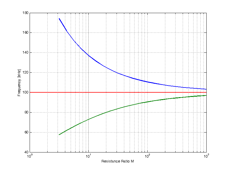
The same results are shown in the table below,
| Res Ratio M | Pole \(p_1\) [kHz] | Pole \(p_2\) [kHz] |
|---|---|---|
| 1 | 38 | 261 |
| 2 | 50 | 200 |
| 5 | 64 | 155 |
| 10 | 73 | 137 |
| 20 | 80 | 125 |
| 50 | 87 | 115 |
| 100 | 90 | 111 |
| 200 | 93 | 107 |
| 500 | 96 | 105 |
| 1000 | 97 | 103 |
The important take away from all of this, is that we must accept a higher output impedance, if we wish to achieve closely spaced poles.
Input Impedance
Here we will derive the worst case input impedance, with the output shorted. We will apply a test current \(I_T\) to the input, and resolve the resulting test voltage \(V_T\). An annotated schematic of the filter is shown below,

Looking into the input of the filter,
\[ V_T = V_x + R_AI_T \]
The intermediate node V_x is,
\begin{align*}
V_x &= I_T (Z_{CA} || R_B ) \\
&= \dfrac{I_T(\frac{1}{sC_A})R_B}{\frac{1}{sC_A} + R_B} \\
&= \dfrac{I_T R_B}{1 + sR_BC_A }
\end{align*}
Substitution,
\begin{align*}
V_T &= \dfrac{I_T R_B}{1 + sR_BC_A } + R_A I_T\\
V_T &= \dfrac{I_T R_B + (1 + sR_BC_A )(R_A I_T)}{1 + sR_BC_A } \\
V_T &= \dfrac{R_A + R_B + sR_AR_BC_A}{1 + sR_BC_A } I_T\\
\end{align*}
Finally the input impedance is
\begin{align*}
Z_{in}(s) &= \dfrac{V_T}{I_T} \\
Z_{in}(s) &= \dfrac{R_A + R_B + sR_AR_BC_A}{1 + sR_BC_A }\\
\end{align*}
Zin has one pole at
\[ p_1 = \dfrac{-1}{R_BC_A} \]
Zin has one zero at
\begin{align*}
z_1 &= \dfrac{-(R_A + R_B)}{R_AR_BC_A}\\
z_1 &= \dfrac{-1}{(R_A||R_B)C_A}\\
\end{align*}
Output Impedance
The output impedance of the filter can be calculated by the short-hand relations for parallel impedances. A schematic representation of the filter is shown below.

The output impedance is then
\[ Z_{out} = Z_{CB} || ( R_B + Z_A ) \]
The parallel combination of \(R_A\) and \(CA\) is as follows,
\[ Z_A = \dfrac{R_A}{1 + sR_AC_A} \]
Substitution yields,
\begin{align*}
Z_{out} &= \dfrac{(\frac{1}{sC_B})(R_B + Z_A)}{\frac{1}{sC_B} + R_B + Z_A} \\
Z_{out} &= \dfrac{R_B + Z_A}{ 1 + sR_BC_B + sZ_AC_B} \\
Z_{out} &= \dfrac{R_B(1 + sR_AC_A) + R_A}{ (1 + sR_AC_A) + sR_BC_B(1 + sR_AC_A) + sR_AC_B} \\
Z_{out} &= \dfrac{R_A + R_B + sR_AR_BC_A}{ 1 + s( R_AC_A + R_BC_B + R_AC_B) + s^2R_AR_BC_AC_B } \\
\end{align*}
The poles and zeros are left as an exercise to the reader.
Example 100 kHz Low-Pass Filter
In order to form a second order low-pass filter with one cut-off frequency, \( R_B \) must be choose to be greater than \( R_A \). As seen from the pole spacing table above, the ratio of \(R_B\) to \(R_A\) dictates how closely the two poles can be placed. For the purposes of an explanatory design, we desire the poles to be \( \pm 10\) % of the nominal cut-off frequency. Consulting the pole spacing table above, we can see that a resistance ratio of 100 satisfies this requirement.
The time-constants \( \tau_A \) and \( \tau_B \) are related to the cut-off frequency as
\[ \tau_A = R_AC_A, \;\;\; \tau_B = R_BC_B \]
\[ \tau = \dfrac{1}{2\pi f_c} \]
Resistor \( R_A \) is chosen arbitrarily as
\[ R_A = 1 \text{ k}\Omega \]
Applying the time-constant relation yields
\begin{align*}
C_A &= \dfrac{1}{2\pi f_c R_A} \\
C_A &= \dfrac{1}{2\pi (100E3)(1E3)} \\
C_A &= 1.59 \text{ nF} \\
\end{align*}
The resistance ratio derived above dictates \(R_B\) to be
\begin{align*}
R_B &= 100 R_A \\
R_B &= 100 \text{ k}\Omega \\
\end{align*}
Finally, the remaining component \(C_B\) is calculated as
\begin{align*}
C_B &= \dfrac{1}{2\pi f_c R_B} \\
C_B &= \dfrac{1}{2\pi (100E3)(100E3)} \\
C_B &= 15.9 \text{ pF} \\
\end{align*}
The complete schematic of the filter is the following

The transfer function of the filter is
\[ H(s) = \dfrac{1}{(2.528\text{E-12}) s^2 + (3.196\text{E-6})s + 1} \]
The two poles of the low-pass transfer function are
\[ |p_1| = 110.6 \text{ kHz} \]
\[ |p_2| = 90.6 \text{ kHz} \]
A bode plot of the resulting filter is shown in the figure below.

Comparing the proposed filter design to that of the ideal case of two cascaded poles each at 100 kHz is shown in the bode plot below. The proposed filter is in reasonable agreement with the ideal case of two poles each at exactly 100 kHz.
The input impedance when the output is left open is shown in the figure below. We can see that for frequencies below 10 kHz, the input impedance appears capacitive (90 degree phase lag) with a capacitance of \( C_A\). Well above the cut-off frequency, the input impedance appears resistive with a value of \(R_A\) = 1 kOhm (60 dBOhm).

The output impedance of the filter is shown in the figure below. At low frequencies, the output impedance appears resitive with a value of \(R_A + R_B \). For higher frequencies, the output impedance is dominated by output capacitor \(C_B\).

H(s)=1(2.528E-12)s2+(3.196E-6)s+1
Calculation of the poles in a 2nd order low pass filter as per your example.
The solution to the above equation id given as 110.6 khz and 90.6khz. How are these figures calculated?
These are not the solutions to the above equation.