The Butterworth filter is an interesting filter in that its origin is based on the desire of a particular magnitude function. Butterworth (S. Butterworth, the Engineer in the 1930’s) demonstrated that the magnitude-squared function of
\[ \left| H\left( j \omega \right)\right|^2 = \dfrac{A^2}{1+\omega^{2n}} \]
has many admirable properties for use as a low-pass filter. To maintain consistency with Butterworth’s original paper and most academic treatments of the Butterworth filter, the filter is described as a prototype filter with unity gain and a cutoff frequency of \( \omega_c = 1 \) rad/s.
-The passband is the frequency spectrum of \( 0 \leq \omega \leq 1 \) rad/s
-The stopband is the frequency spectrum of \( \omega > 1 \)
-At the corner frequency \( \omega_c = 1\) rad/s, the magnitude response is always
\[|H(j\omega_c)| = \frac{1}{\sqrt{2}}=\;\; – 3 \text{ dB, for any filter order n.}\]
-Past the corner frequency \(\omega_c\) the magnitude response declines at a rate of \(-20 n \) dB/decade
-The magnitude response over frequency is monotonic (i.e. flat or decreasing) , thus no ripple.
Continue reading “Butterworth Filter”

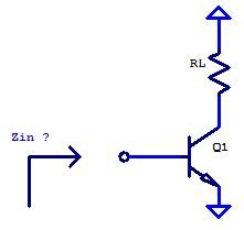
 amplifier.") In this post, a circuit equivalent model of the output impedance of a common-emitter amplifier will be developed. To begin, a low-frequency non-reactive model of the output resistance of a common-emitter (CE) amplifier will be solved. Proceeding models will include the capacitive elements of a CE amplifier. Separating the High-Frequency (HF) model into two distinct cases will allow for circuit analysis that is reasonable to perform by hand. The first HF model will be for when the base is ac-grounded and the emitter see a degeneration resistor. A second HF model is developed with a grounded emitter and with source resistance to the input (base) terminal. Concluding the post with a spice simulation to compare/validate the circuit equivalent models developed. The desired outcome of this post is to gain an intuition into what “it looks like” electrically speaking into the output of a CE amplifier.
In this post, a circuit equivalent model of the output impedance of a common-emitter amplifier will be developed. To begin, a low-frequency non-reactive model of the output resistance of a common-emitter (CE) amplifier will be solved. Proceeding models will include the capacitive elements of a CE amplifier. Separating the High-Frequency (HF) model into two distinct cases will allow for circuit analysis that is reasonable to perform by hand. The first HF model will be for when the base is ac-grounded and the emitter see a degeneration resistor. A second HF model is developed with a grounded emitter and with source resistance to the input (base) terminal. Concluding the post with a spice simulation to compare/validate the circuit equivalent models developed. The desired outcome of this post is to gain an intuition into what “it looks like” electrically speaking into the output of a CE amplifier.